The Timeseries Viewer
The Timeseries Viewer can display time series data as line graphs. Like the Timeline and Waveform viewer, it has a horizontal time-scale bar, a red vertical crosshair indicating the media time and a light blue rectangle to highlight the selected time interval. It has also the same zoom and pan options.
It can display multiple “track panels” and each track panel can display multiple “tracks”. Track panels and tracks can be added and removed via a popup menu. Each track panel derives its value range (vertical axis) from one of the tracks. The viewer has a facility to transfer data from a track to annotation values. Based on the time intervals of the annotations on a chosen (time-alignable) tier, the minimum, maximum or average of the data within these intervals of the selected track will be copied to annotations on a dependent, symbolically associated tier.
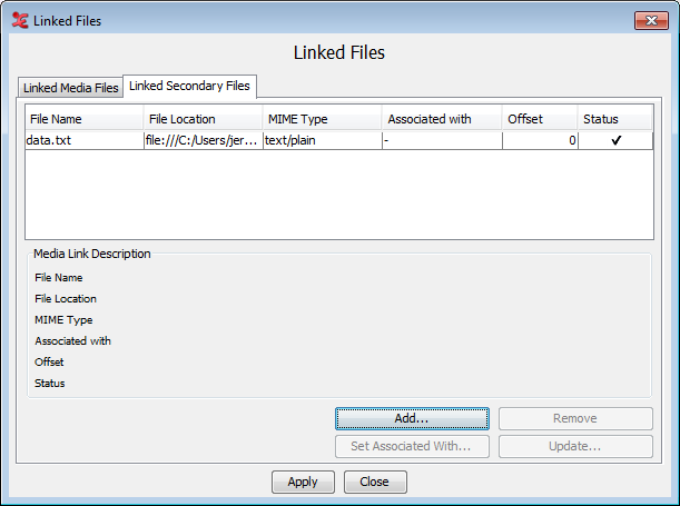
The Timeseries Viewer will be created after at least one supported timeseries data file has been associated to the transcription via menu and then the tab “Linked Secondary Files”. These data files can be synchronized to the media files in the “Media Synchronization Mode”.
![[Note]](images/note_1855015319.png) | Note |
|---|---|
Currently supported file formats are CSV/Tab delimited text files, Praat .PitchTier and .IntensityTier files, a proprietary .log file produced by MPI CyberGlove software and a special kind of plain text (.txt) file, containing a time-value pair on each line. Software developers can add support for other formats by implementing a Service Provider Interface (more information can be found in the source code release notes). |
Figure 99. Linking timeseries data files
 |
Displaying data from an already linked CSV/Tab delimited text file in the Timeseries Viewer is done as follows:
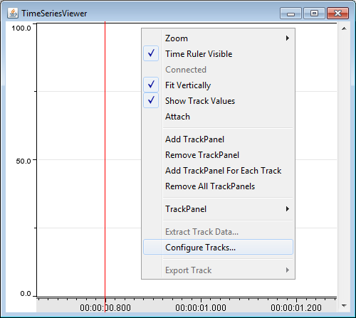
Right click in the Timeseries Viewer and select .
Figure 100. Timeseries Viewer popup menu
If you have more than one file linked as secondary file, choose the file you wish to use from the pull down menu that is now displayed and click .
In the next window you see a sample table with several lines and columns of the chosen file. At least one of the columns must contain time data. Select that column by selecting the appropriate column number at
Time Column
                  Index
. If the time codes have a fixed interval, you can check the optionContinuous Rate. Its underlying purpose is to speed up the calculations for displaying a data track.Figure 101. Timeseries Viewer: Configure tracks
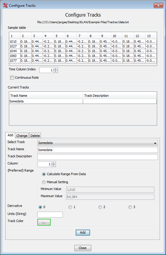
After you have selected a column as the time column, you can begin creating tracks. On the Add tab, enter a
Track Nameand optionally aTrack Description. Select the number of the column in the data that you want to use for this track and specify the range for the vertical axis. This can be automatically calculated by selectingCalculate Range From Dataor it can be set manually by selectingManual Settingand entering theMinimum ValueandMaximum Value.The
Derivativeoption allows you to display the first, second or third derivative of your data. Derivatives are useful if we are, for example, dealing with data that represent the position of an object, but we wish to see the velocity of that object. Because velocity is the first derivative of position, we would select1. In this example, 2 would represent the acceleration and 3 the rate of change of acceleration, also called jerk or jolt.Enter the units of your data, for instance meters for position or Pascal (Pa) for pressure at the
Units
                  (String)
option. Select a color by clicking the colored box atTrack Color.Finally click the button. The track is now added to the list of Current Tracks which is above the Add tab. Continue adding tracks for each column of data you wish to display. After adding tracks, click on the button.
To display the track right click on the Timeseries Viewer again. Select to add a new track panel. Right click the new track panel and select . A list of not yet displayed tracks is displayed. Click one to add it to the track panel.
The other options from the popup menu are:
Zoom: zoom in and out horizontally.
Time Ruler Visible: hides or shows the time scale bar.
Connected:
Fit Vertically: fit the track panel(s) vertically to the Timeseries Viewer window.
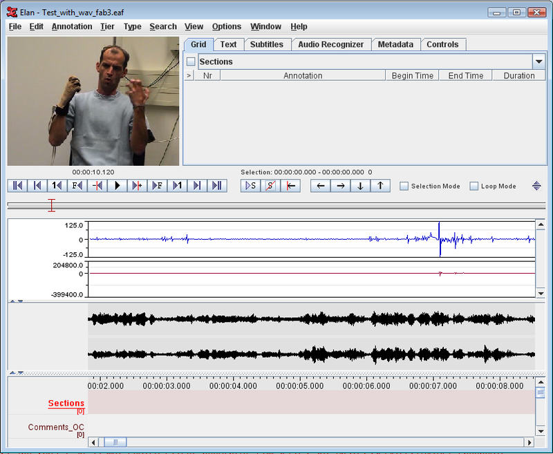
Attach: attaches of detaches the Timeseries Viewer to the main window.
Figure 102. Timeseries viewer in the main window
Add TrackPanel: create a track panel
Remove TrackPanel: remove current track panel.
Add TrackPanel For Each Track: create a track panel for each of the existing tracks.
Remove All TrackPanels: remove all track panels form the Timeseries Viewer window.
TrackPanel > Set Range For Panel: set the vertical range to the range specified for a track.
TrackPanel > Remove Track: remove a track from the current track panel.
TrackPanel > Add All Tracks: add all tracks to the current track panel.
TrackPanel > Remove All Tracks: remove all tracks from the current track panel.
Extract Track Data: Extract data from a track and add it to a tier. This process consists of two steps:
Selection of a source and a destination tier. The annotations of the source tier provide the segments for which to extract data from a track. The destination tier should be a (Symbolic Association) dependent tier of the source tier. The numerical values that have been extracted per segment will be stored in dependent annotations on the destination tier.
Selection of the track to extract data from. There are a number of options for what has to be extracted (calculated):
Figure 103. The Extract Track Data window
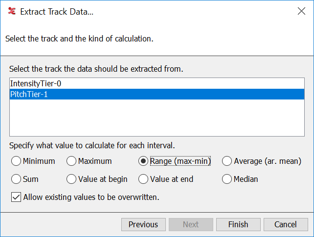
Minimum - the smallest value found in the interval
Maximum - the largest value in the interval
Range - the maximum minus the minimum value in the interval
Average (arithmetic mean) - the average of all values in the interval
Sum - the total of all values in the interval
Median - the median of all values in the interval
The value at the begin of the segment
The value at the end of the segment
The checkbox allows to determine whether existing annotations on the destination tier may be overwritten or not.